Classification Model Builder
Description
This step lets you build a classification model based on training data. One column or attribute of your data set can typically be considered as one feature. Features should ideally be independent. Features are also referred to as dimensions. Value which you want to predict is called label. This step can be used to build the model when features are either of Number type or String type or mixed.
Configurations
| No. | Field Name | Description |
|---|---|---|
| Row Handling | ||
| 1 | Step name | Used to specify the name of the step. The step name should be unique within the workflow. |
| 2 | Number of Rows to Process | Can have following two values. - All - Batch Governs if all the rows of dataset are passed in one shot or they are batched. Typically if you are building model on a very large dataset, you can use Batch row processing. |
| 3 | Size | It has meaning only when Batch is selected for ‘Number of Rows to Process’. If your dataset has 50,000 rows, 1,000 can be a good batch size candidate. Data Model Location |
| 4 | Build using AE Model Version | Select the Python version you will use for building the model. Note: The Python version you select must be same as the version you have saved in the python folder or added to the environment variable path. |
| 5 | File name | Used to specify name and location of the file which will contain the model |
| Algorithm | ||
| 6 | Algorithm | Used to specify algorithm to be used for building the model. Step supports following algorithms - Linear SVC - SVC - Decision Tree Classifier - Random Forest Classifier - Logistic Regression - Multinomial NB - SGD Classifier - K Neighbors Classifier |
| 7 | Algorithm Parameters* | Based on the algorithm selected, corresponding algorithm parameters are shown. These are described in the last table of this plugin description. |
| Fields | ||
| 1 | Name | Name of the field |
| 2 | Incoming Type | Used to specify data type of the field. It can either be Number or String |
| 3 | Text Processing | All the classification algorithms work on vectors of numbers. Fields which are of type String need to be converted internally to numeric vectors and this cell lets you specify all the Text Processing attributes on that field. This cell can be clicked only for fields with String data type. Ensuing dialog when you click on it has two tabs. - First tab lets you specify one or more text processing options. - Remove punctuation: removes standard punctuation marks from the text - Remove Stop Words: removes stop words like ‘the’, ‘as’, ‘in’ etc. - Additional Stop Words: this lets you choose a simple text file where every additional stop word is there on a separate line. These are your domain specific stop words. - Lemmatization: this converts words like mice to mouse, houses to house etc. - Stemming: this gets stem of the word no matter what word form is used in the text. So going, went, goes etc. would be converted to go - Second tab lets you Test your text processing options. In the text box next to ‘Value:’ you can type any text. Clicking on ‘Test’ button will give you the text in the text box next to ‘Result:’ taking into account text processing options you have selected. |
When you are processing a feature of type string, as mentioned in ‘Text Processing’ section of above table, this feature needs to be converted into numeric features. Text Vectorization Tab governs how all string features get converted into numeric features. An n-gram is a contiguous sequence of n items from a given sample of text or speech. Table below shows how internally a string gets tokenized given different values of n-gram
| No. | String | N Gram Start/End | Tokens |
|---|---|---|---|
| 1 | Weather today is good | 1-1 | 'Weather', 'today', 'good' |
| 2 | Weather today is good | 1-2 | 'Weather', 'today', 'good', 'Weather today', 'today good' |
| 3 | Weather today is good | 1-3 | 'Weather', 'today', 'good', 'Weather today', 'today good', 'Weather today good' |
| 4 | Weather today is good | 2-3 | 'Weather today', 'today good', 'Weather today good' |
*is treated as stop word and not considered
| No. | Field Name | Description |
|---|---|---|
| Text Vectorization Tab | ||
| 1 | N Gram start | Should be a numeric value with minimum of 1 |
| 2 | N Gram end | Should be a numeric value greater than or equal to N Gram start |
| 3 | Vectorization | N-Gram operation tokenizes input string feature. Vectorization is the operation where these tokens are converted to numeric features which are needed by the algorithms. There are three types of vectorizers supported - Count Vectorizer: It counts the number of times a token shows up in the document and uses this value as its weight. - Tfidf Vectorizer: TF-IDF stands for “term frequency-inverse document frequency”, meaning the weight assigned to each token not only depends on its frequency in a document but also how recurrent that term is in the entire corpora. - Hashing Vectorizer: It is designed to be as memory efficient as possible. Instead of storing the tokens as strings, the vectorizer applies the hashing trick to encode them as numerical indexes. The downside of this method is that once vectorized, the features’ names can no longer be retrieved. |
| No. | Field Name | Description |
|---|---|---|
| Evaluation Tab | ||
| 1 | Evaluation Type | Choose an Evaluation Algorithm Type from the drop down list as seen in the snapshot below, - None – Choose None if Evaluation is not needed - Train/Test Split – This Evaluation Algorithm splits the data into Train and Test as per parameters specified below. The data we use is usually split into training data and test data. The training set contains a known output and the model learns on this data in order to be generalized to other data later on. We have the test dataset (or subset) in order to test our model’s prediction on this subset. - Stratified k-Fold Cross-Validation – In this Evaluation Algorithm we split our data into k different subsets (or folds). We use k-1 subsets to train our data and leave the last subset (or the last fold) as test data. We then average the model against each of the folds and then finalize our model. After that we test it against the test set. |
| 2 | Test Percentage | For Train/Test Split: Data Types allowed: default value float, int or None, optional (default=None) - If float, should be between 0.0 and 1.0 and represent the proportion of the dataset to include in the test split. - If int, represents the absolute number of test samples. - If None, it will be set to 0.25. |
| 3 | Number of Folds | For Stratified k-Fold Cross-Validation: Data Types allowed: int, default=3 - Must be at least 2. Default value is 3. |
| 4 | Random State | For Train/Test Split: Data Types allowed: int, RandomState instance or None, optional (default=None) - If int, random_state is the seed used by the random number generator; - If RandomState instance, random_state is the random number generator; - If None, the random number generator is the RandomState instance used by np.random. |
| 5 | Shuffle | For Stratified k-Fold Cross-Validation: Data Types allowed: boolean, optional (default=True) - Whether to shuffle each class’s samples before splitting into batches. |
| 6 | Evaluation Output File Name | Absolute html report output file path. For Train/Test Split: 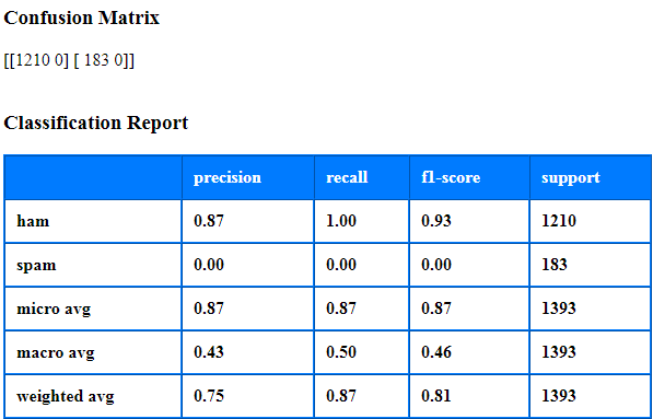 For Stratified k-Fold Cross-Validation: 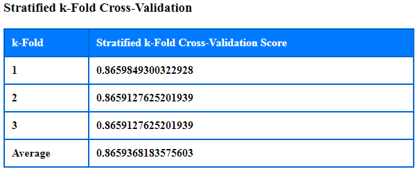 |
| 7 | Add output filename to result | Enable checkbox to display downloadable link of html report output file on AE portal. |
*The following rows list the algorithms along with a description and snapshots of corresponding parameters. The right hand column has the description of these parameters.
| Algorithm Description | Algorithm Parameter Description | |
|---|---|---|
| 1 | Linear SVC: Firstly, by any chance if data is linearly separable in any dimension(s) of the features, undoubtedly, one should choose Linear SVM or Logistic Regression. Even though one might achieve similar results with the other complex algorithms, they are not recommended for two reasons; 1- Complexity often leads to more computation time 2- Overfitting Linear SVM is an extremely fast machine learning (data mining) algorithm for solving multiclass classification problems from ultra large data sets.  | Loss: It specifies the loss function. ‘hinge’ is the standard SVM loss (used e.g. by the SVC class) while ‘squared_hinge’ is the square of the hinge loss. In machine learning, loss function measures the quality of your solution, while penalty function is mainly responsible to minimize the misclassification error (It imposes some constraints on your solution for regularization). C is the penalty parameter of error term. It maximizes the kernel margin while keeping the misclassification error minimum. C is 1 by default and it’s a reasonable default choice. It works well for the majority of the common datasets. If you have a lot of noisy observations in the data set you should decrease it. Lower the C value, better the results are for noisy data and exactly opposite in case of clean data. max_iter (int, default=1000) is the maximum number of iterations to be run for convergence. |
| 2 | SVC: The objective of a Linear (kernel) SVC (Support Vector Classifier) is to fit to the training data provided, returning a "best fit" hyperplane that divides, or categorizes, your training data. From there, after getting the hyperplane, you can then feed some features to your classifier to see what the "predicted" class is.  SVC Use Cases: - Predicting if student passes/fails based on previous exam scores Used mainly with numerical data and when there is a need for high classification accuracy without compromising on efficiency. | Kernel (string, optional (default=’rbf’)) Specifies the kernel type to be used in the algorithm. It must be one of ‘linear’, ‘poly’, ‘rbf’, ‘sigmoid’, precomputed’ or a callable. If none is given, ‘rbf’ will be used. If a callable is given it is used to pre-compute the kernel matrix from data matrices; that matrix should be an array of shape (n_samples, n_samples). Currently, the plugin supports ‘linear’, ‘poly’ and ‘rbf’ as explained below, i. Linear Kernel works well only when the data is linearly separable (in any dimension of feature space). This hyperplane which is a learned model can be used for prediction. ii. RBF kernel of SVM especially might do a decent job in most of the other datasets that are non-linear. RBF is widely used kernel with Non Linear datasets. iii. Poly kernel is suitable if data is separable by higher order functions. Practical usage or benefits are pretty less. Hence it is not the most commonly used kernel. C is the penalty parameter. It maximizes the margin while keeping the misclassification error minimum. C is 1 by default and it’s a reasonable default choice. It works well for the majority of the common datasets. If you have a lot of noisy observations in the data set you should decrease it. Lower the C value, better the results are for noisy data and exactly opposite in case of clean data. Probability: This is a Boolean and optional. Choose True or False from the drop down list (default=False). It is about whether to enable probability estimates. This must be enabled prior to calling fit (Fit the SVM model according to the given training data). |
| 3 | Decision Tree Classifier: It is one of the predictive modeling approaches used in machine learning. Decision tree learning uses a decision tree to go from observations about an item to conclusions about the item's target value. Decision Tree Classifier Use Cases: - Decision Tree Classifier /Random Forest Classifier are predominantly used in recommendation systems/problem. max_depth: It is an integer or None (default=None). max_depth is optional. The maximum depth of the tree. If None, then nodes are expanded until all leaves are pure. | max_depth: It is an integer or None (default=None). max_depth is optional. The maximum depth of the tree. If None, then nodes are expanded until all leaves are pure. |
| 4 | Random Forest Classifier: Random Forest Classifier is ensemble algorithm. Ensembled algorithms are those which combine more than one algorithms of same or different kind for classifying objects. Random Forest is a flexible, easy to use machine learning algorithm that produces, even without hyper-parameter tuning, a great result most of the time. It is also one of the most used algorithms, because it’s simplicity and the fact that it can be used for both classification and regression tasks. RFC mainly overcomes some of the limitations that Decision Tree Classifiers has: - Only One tree and one decision for the entire data as well as feature set Overfitting. - Computational efficiency(not all cases) - Improper decision rules (in some cases) - Random Forest Classifier Use Cases: - Decision Tree Classifier /Random Forest Classifier are predominantly used in recommendation systems/problems. - Predicting the risk(high/low/medium) of a loan application - Predicting social media share scores etc. | max_depth int or None, optional (default=None). It is the maximum depth of each tree in the Random Forest. If None, then nodes are expanded until all leaves are pure. |
| 5 | Logistic Regression: A classification model that uses a sigmoid function to convert a linear model's raw prediction into a value between 0 and 1. You can interpret the value between 0 and 1 in either of the following two ways: - As a probability that the example belongs to the positive class in a binary classification problem. As a value to be compared against a classification threshold. If the value is equal to or above the classification threshold, the system classifies the example as the positive class. Conversely, if the value is below the given threshold, the system classifies the example as the negative class Logistic Regression Use Cases: - Classifying words as nouns, pronouns, and verbs. - Weather forecasting applications for predicting rainfall and weather conditions. | C is the penalty parameter. It maximizes the margin while keeping the misclassification error minimum. C is 1 by default and it’s a reasonable default choice. It works well for the majority of the common datasets. If you have a lot of noisy observations in the data set you should decrease it. Lower the C value, better the results are for noisy data and exactly opposite in case of clean data. max_iter (int, default=1000) is the maximum number of iterations to be run for convergence. |
| 6 | Multinominal NB: Naive Bayes: The Naive Bayes classifier is a simple probabilistic classifier which is based on Bayes theorem with strong and naïve independence assumptions. MultinomialNB: A variant of Naive Bayes which is mainly used for text classification. This variation, estimates the conditional probability of a particular word/term/token given a class as the relative frequency of term t in documents belonging to class c. The multinomial Naive Bayes classifier is suitable for classification with discrete features (e.g., word counts for text classification). The multinomial distribution normally requires integer feature counts. However, in practice, fractional counts such as tf-idf (term frequency–inverse document frequency) may also work. Multinomial NB Use Cases: - illness forecast - Grouping information (blog posts etc.) | alpha (float, optional (default=1.0)) Additive (Laplace/Lidstone) smoothing parameter (0 for no smoothing). |
| 7 | SGD Classifier: Gradient descent is an optimization algorithm used to find the values of parameters (coefficients) of a function (f) that minimizes a cost function (cost). Gradient descent is best used when the parameters cannot be calculated analytically (e.g. using linear algebra) and must be searched for by an optimization algorithm. In situations when you have large amounts of data, you can use a variation of gradient descent called stochastic gradient descent. Stochastic Gradient Descent (SGD) is a simple yet very efficient approach to discriminative learning of linear classifiers under convex loss functions such as (linear) Support Vector Machines and Logistic Regression.  SGD Classifier Use Cases: SGD has been successfully applied to large-scale and sparse machine learning problems often encountered in text classification and natural language processing. | max_iter (int, default=1000) is the maximum number of iterations to be run for convergence. In machine learning, loss function measures the quality of your solution, while penalty function is mainly responsible to minimize the misclassification error (It imposes some constraints on your solution for regularization). penalty: string, ‘l1’ or ‘l2’ (default=’l2’) Specifies the norm used in the penalization. The ‘l2’ penalty is the standard used in SVC. The ‘l1’ leads to coef_vectors that are sparse. **loss: **It specifies the loss function. Options are hinge, log, modified_huber, squared_hinge, perception. |
| 8 | K Neighbours Classifier: KNN is not really a training algorithm. K nearest neighbors is a simple algorithm that stores all available cases and classifies new cases based on a similarity measure (e.g., distance functions). In pattern recognition, the k-nearest neighbors algorithm (k-NN) is a non-parametric method used for classification and regression. In both cases, the input consists of the k closest training examples in the feature space. K Neighbors Classifier Use Cases: Retail analytics (Finding a similar product which customer is likely to buy or put in the basket). | n_neighbours: It defines the no. of nearest neighbors to be considered for prediction based on the distance. |
Limitations: User may get a value conversion error in the scenario where the count of fields in the Microsoft Excel Input step differs from those that need to be passed to the ML: Model Builder step. The error occurs because of incorrect data type conversion in the Microsoft Excel Input step. The workaround is:
- Ensure that the Microsoft Excel Input step has the same fields as that required in the ML: Model Builder step. OR
- Ensure data type of all fields is String.
Glossary:
- **Loss:**A measure of how far a model's predictions are from its label. Or, to phrase it more pessimistically, a measure of how bad the model is. To determine this value, a model must define a loss function. For example, linear regression models typically use mean squared error for a loss function, while logistic regression models use Log Loss.
- Penalty: A type of regularization that penalizes weights in proportion to the sum of the absolute values of the weights.
- Kernel: A classification algorithm that seeks to maximize the margin between positive and negative classes by mapping input data vectors to a higher dimensional space. For example, consider a classification problem in which the input dataset has a hundred features. To maximize the margin between positive and negative classes, a KSVM could internally map those features into a million-dimension space. KSVMs uses a loss function called hinge loss.
- Conversion: A convergence of a model's predictions to its labels.